How nbdev helps us structure our data science workflow in Jupyter Notebooks

Jupyter notebooks have been rightly praised for making it very easy and intuitive to experiment with code, visualize results and describe your process in nicely formatted markdown cells. In our work as data scientists and Machine Learning Engineers at 20tree.ai, we are using notebooks all the time and they are a great tool in our toolbox. However, there are some downsides that we experience using notebooks in our workflow. For one thing, working in notebooks often results in unstructured, badly documented and untested code that takes a lot of time to transport into a proper codebase. Also, version control in Jupyter Notebooks is a disaster and involves large changes in each commit that are hard to traceback.

Nbdev solves many of these issues by making it very easy to transform Jupyter notebooks into proper python libraries and documentation. It incentives us to write clear code, use proper Git version control and document and test our codebase continuously. At the same time preserving the benefits of having interactive Jupyter notebooks in which it is easy to experiment. Using nbdev has improved our workflow significantly and perhaps it can do the same for you!

What is nbdev?

nbdev is a library created by fast.ai that forms the missing link between the data exploration of Jupyter notebooks and programming an actual codebase that produces high-quality software. In short, nbdev provides a framework for:

• Exporting selected notebook cells into a Python library

• Automatically generating documentation based on function signatures and notebook cells

• Running notebook cells as unit tests.

Of course, it has many more features that you can find at nbdev.fast.ai or by reading the nbdev launch post, but these are the ones we make the most use of. In addition, nbdev provides utilities for stripping notebook metadata and handling merge conflicts, both greatly improving development cycles (and general quality of life 🙂 ) when checking notebooks into a git repository.

Every notebook that has a #default_exp tag at the start, gets exported to a Python module. Automatically using best practices such as defining which functions get imported when you do import * by setting __all__ = [‘function1’, ‘functon2’, …].

The magic of nbdev is that it doesn’t actually change programming that much; you add a # export or # hide tag to your notebook cells once in a while, and you run nbdev_build_lib and nbdev_build_docs when you finish up your code. That’s it! There’s nothing new to learn, nothing to unlearn. It’s just notebooks. More than anything, nbdev encourages us to write cleaner notebooks with a clear separation between code (the cells that get exported) and experimentation, visualization and testing (the cells that don’t get exported). As a result, our notebooks are more readable, and easier to share among the whole team. As a wise (wo)man once said, the real nbdev was inside of us all along.

index.ipynb with the generated documentation from this notebook next to it.

Why do we use it?

As data scientists, much of our work involves — as you might expect — data. This means loading data, transforming data, combining data, and at some point actually using that data. Especially in the transforming and combining stages, it’s critical to ensure that no mistakes slip in. If you are trying to train a neural network for semantic segmentation but your segmentation map is shifted by a few pixels, your data is essentially invalid. Worse yet, valuable time is often lost trying to get some code or machine learning models to work, while minor typos have sneaked in such small, stupid, but bothersome bugs. Because notebooks are run iteratively through cells it’s almost like you’re debugging while coding. Errors are much quicker caught this way. Here at 20tree.ai, we mostly work with georeferenced (satellite) data. When different parts of your data are projected in different coordinate reference systems, it (again) becomes very easy for mistakes to slip in.

When developing new code, a pretty standard pattern for us consist of the following:

1. Small functions are written in a Jupyter notebook. The notebook is used to visually inspect the output and to informally test that the code behaves as expected;

2. The functions get copy-pasted into a proper codebase;

3. The original notebooks are scattered to the wind;

4. Code gets changed over time, maybe a mistake slips in. When asking for more details on a bit of code, someone points to some file called Untitled_v3_better_labels2.ipynb with the comment “it’s probably very outdated though”.

With nbdev, we can nip this whole sequence in the bud. You write your code in a Jupyter notebook and that’s it. You’re done, because the notebook is the proper codebase! The main code cells are exported to the library and the output of some cells forms the visual explanation as well as unit tests — that you’d have to make generally separately otherwise — that are automatically run when pushing the notebook to Github. So while iteratively coding documentation and testing are (almost) entirely free. For example, after implementing data augmentation, you’re surely going to visualize the outputs to ensure that the data looks as you would expect and, just as importantly, that the labels are similarly transformed. With nbdev, this visualization is simply in your codebase, right below the function definition:

These tests can also very easily be used in your Github continuous integration pipeline, making it very easy to do proper checks before merging some new code into your existing codebase.

The fact that your entire codebase is living in notebooks also means that when something is not working as expected, it is very easy and intuitive to debug. You can quickly change something and see how it affects the output.

Best practices we found

In the past month that we have been using nbdev in our workflow, we have developed some best practices.

Use test flags such as server, cuda or slow that can be set in your settings.ini by setting tst_flags = server|cuda|slow. Cells that are given this flag will not be run during testing unless specifically requested. This can be useful if, for example, you are running a function using a large dataset that is only available on the server.

Add a #server the start of the cell to avoid it being run during testing.

Be extra careful to make clean commits as changes in Jupyter Notebook are not very readable on Github. The nbdev command-line functions nbdev_fix_merge (which splits merge conflicts) and nbdev_clean_nbs(which removes metadata from your notebooks) are very useful for this. Also, we use git add -p to select specific changes in a notebook to be added to the commit. If you are using Jupyter Lab you can also install the Git extension to view changes.

You can also use the Jupyter Lab Git extension to directly view changes in your Notebooks or you can use the Github ReviewNB app to view all the changes for a particular PR (paid for private repositories)

Always add some sanity checks after defining a function, since it is automatically added as a test this makes your code much more reliable, it also shows the user the expected output in the documentation. If you don’t want a test to appear in your documentation you can simply add #hide at the beginning of the cell (the test will still be run). Use nbdev_test_nbs to test all the Notebooks locally.

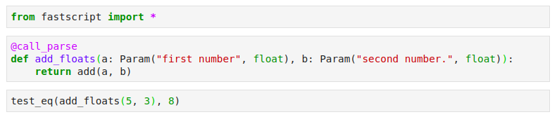
You can use test_eq() to quickly run a test while at the same time showing the expected output in the docs.

For defining command-line functions, we use fastscript, another great library by fast.ai, which makes it possible to define a command-line function that can also be run as a regular function, making it very convenient to test in the notebook as well. You can add your command line functions by adding them in settings.ini(separated by spaces).

console_scripts = math_add=math.core:add_floats

Many of the awesome widgets that make Jupyter Notebooks so powerful can be displayed in the documentation, as long as it can be rendered as an HTML output (which is possible for most widgets). For example, we can use folium to render a map with a GeoJSON layer in our documentation.

Authenticated nbdev docs

The only real problem we encountered with using nbdev for generating our documentation is that some of our documentation contains sensitive customer data and other information that we want to keep secure, which means that we don’t want to host it on a public Github pages website.

To solve this issue we use https://github.com/benbalter/jekyll-auth which makes it very easy to host a Jekyll website on Heroku using Github authentication. The beauty of this solution is that you can immediately give your entire Github organization or Github team access to the documentation. For the full details on implementing this, check out our other blog post on Auto-Generated Authenticated Python Docs using nbdev and Heroku).

Conclusion

Even though we only just started using nbdev, it has already proven to be extremely useful to us. The idea of building libraries entirely from within Notebooks is truly paradigm-shifting and makes us not only more effective both individually and as a team, but also allows us to be much more inter-disciplinary, through feature-rich, visual, and well-documented code.

Thanks to Indra den Bakker and Roelof Pieters.